Intro
In this post, we will dive deeper into the {purrr} package. We will explore purrr::nest() %>% dplyr::mutate(), which is an alternative to the split() function in the base-R. Moreover, we will see how the combination of purrr::nest() %>% dplyr::mutate() with purrr::map2_*() or purrr::pmap_*() can be a powerful tool in functional programming.
The data we are going to use was narrowed down to the following variables of interest for the current post. For more information about data, please checkout here.
| Variable Code | Type | Description |
|---|---|---|
year |
String | The year that data was collected |
id |
Integer | Respondent ID |
age |
Integer | Age in years at screening |
gender |
Category | Gender: male or female |
race_ethnic |
Category | Race/Hispanic origin: mexican-american, non-hispanic-black, non-hispanic-white, other-hispanic, other-race |
hh_food_secure |
Integer | Household food security category over last 12 months |
age_group |
Binary | Age group: adult(20+) or child(6-19) |
educ |
Integer | Education level for adults 20+ and children/youth 6-19 |
Let’s take a look at the dataframe.
head(df)
# A tibble: 6 x 8
  year         id   age gender race_ethnic        hh_food_secure
  <chr>     <dbl> <dbl> <fct>  <fct>                       <dbl>
1 1999-2000     2    77 male   non-hispanic-white              1
2 1999-2000     3    10 female non-hispanic-white              1
3 1999-2000     5    49 male   non-hispanic-white              1
4 1999-2000     6    19 female other-race                      1
5 1999-2000     8    13 male   non-hispanic-white              1
6 1999-2000     9    11 female non-hispanic-black              2
# … with 2 more variables: age_group <fct>, educ <dbl>
split vs. nest
We are interested in how food security changes over time, separated by gender and age group (child and adult). For the first step, we want to split the dataframe into lists with split as the following. However, the three grouping variables (gender, age group, and year) are merged together into one column. This is less desirable because we will need each of these variables for later.
split_df = split(df, list(df$gender, df$age_group, df$year))

head(split_df$`female.adult.1999-2000`)
# A tibble: 6 x 8
  year         id   age gender race_ethnic        hh_food_secure
  <chr>     <dbl> <dbl> <fct>  <fct>                       <dbl>
1 1999-2000    15    38 female non-hispanic-white              1
2 1999-2000    16    85 female non-hispanic-black              4
3 1999-2000    20    23 female mexican-american                1
4 1999-2000    24    53 female non-hispanic-white              1
5 1999-2000    25    42 female non-hispanic-white              1
6 1999-2000    34    38 female non-hispanic-black              3
# … with 2 more variables: age_group <fct>, educ <dbl>
Equivalently, we can also use nest from the {purrr} package as the following:
nest_df = df %>%
  group_by(year, age_group, gender) %>%
  nest()

head(nest_df)
# A tibble: 6 x 4
# Groups:   year, gender, age_group [6]
  year      gender age_group data
  <chr>     <fct>  <fct>     <list>
1 1999-2000 male   adult     <tibble [2,211 × 5]>
2 1999-2000 female child     <tibble [1,698 × 5]>
3 1999-2000 male   child     <tibble [1,744 × 5]>
4 1999-2000 female adult     <tibble [2,534 × 5]>
5 2001-2002 male   adult     <tibble [2,384 × 5]>
6 2001-2002 female adult     <tibble [2,669 × 5]>
These two approaches end with very similar results, except gender, age_group, and year are maintained with its original structure with nest() but not with split().
Moreover, with nest(), we can manipulate the data frame within each row while save the output as another column. We will calculate within each gender, age group and year, how food security changes with age. (If you find the map() function confusing, I encourage you take a look at this post.)
model_df = nest_df %>%
  mutate(n = map_dbl(data, nrow),
         m1 = map(data, ~lm(hh_food_secure ~ age, data = .x)),
         coefs = map(m1, coef),
         intercept = map_dbl(coefs, 1),
         slope = map_dbl(coefs, 2))

head(model_df)
# A tibble: 6 x 9
# Groups:   year, gender, age_group [6]
  year      gender age_group data            n m1     coefs  intercept
  <chr>     <fct>  <fct>     <list>      <dbl> <list> <list>     <dbl>
1 1999-2000 male   adult     <tibble [2…  2211 <lm>   <dbl …  1.599724
2 1999-2000 female child     <tibble [1…  1698 <lm>   <dbl …  1.573725
3 1999-2000 male   child     <tibble [1…  1744 <lm>   <dbl …  1.691323
4 1999-2000 female adult     <tibble [2…  2534 <lm>   <dbl …  1.582938
5 2001-2002 male   adult     <tibble [2…  2384 <lm>   <dbl …  1.752420
6 2001-2002 female adult     <tibble [2…  2669 <lm>   <dbl …  1.703107
# … with 1 more variable: slope <dbl>
first figure
Let’s take a look at how the slope change with time:
model_df %>%
  ggplot(aes(x = year, y = slope, color = age_group, group = age_group)) +
  geom_line(size = 1.5) +
  facet_wrap(~gender, nrow = 2) +
  theme(legend.position = 'bottom') +
  labs(y = 'Slope: Age and Food Security',
       x = 'Year',
       color = 'Age Group')

From the figure, we can see that for adults, the slope is consistently negative across all time. In other words, as people age, the food security score decreased. However, for children, the food security increased dramatically recently, especially since 2010s. What if we want to dig deeper and see how age influences children’s food security within each year for different gender?
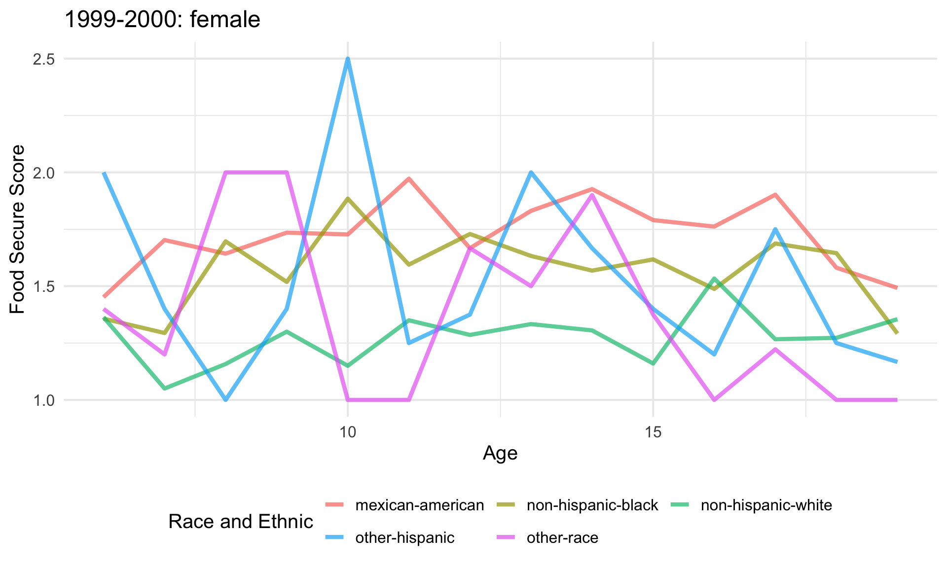
Let’s start with only one row of data:
child_model_df = model_df %>% filter(age_group == 'child')

plotting <- function(df, gender, year = NULL){

  p = df %>%
    group_by(age, race_ethnic) %>%
    summarise(m = mean(hh_food_secure),
              sd = sd(hh_food_secure)) %>%
    ggplot(aes(x=age,
               y=m,
               color = race_ethnic))+
    geom_line(alpha = 0.7, size = 1.5) +
    theme(legend.position = 'bottom')+
    labs(x = 'Age',
         y = 'Food Secure Score',
         color = 'Race and Ethnic') +
    guides(color=guide_legend(nrow=2, byrow=TRUE))

  if(missing(year)){
    p = p + labs(title = gender)
  }else{
    p = p + labs(title = paste(year, gender, sep = ": "))}

  p

  }

# make sure the funtion works for one row of data.
plotting(child_model_df$data[[1]],
         child_model_df$gender[[1]],
         child_model_df$year[[1]])
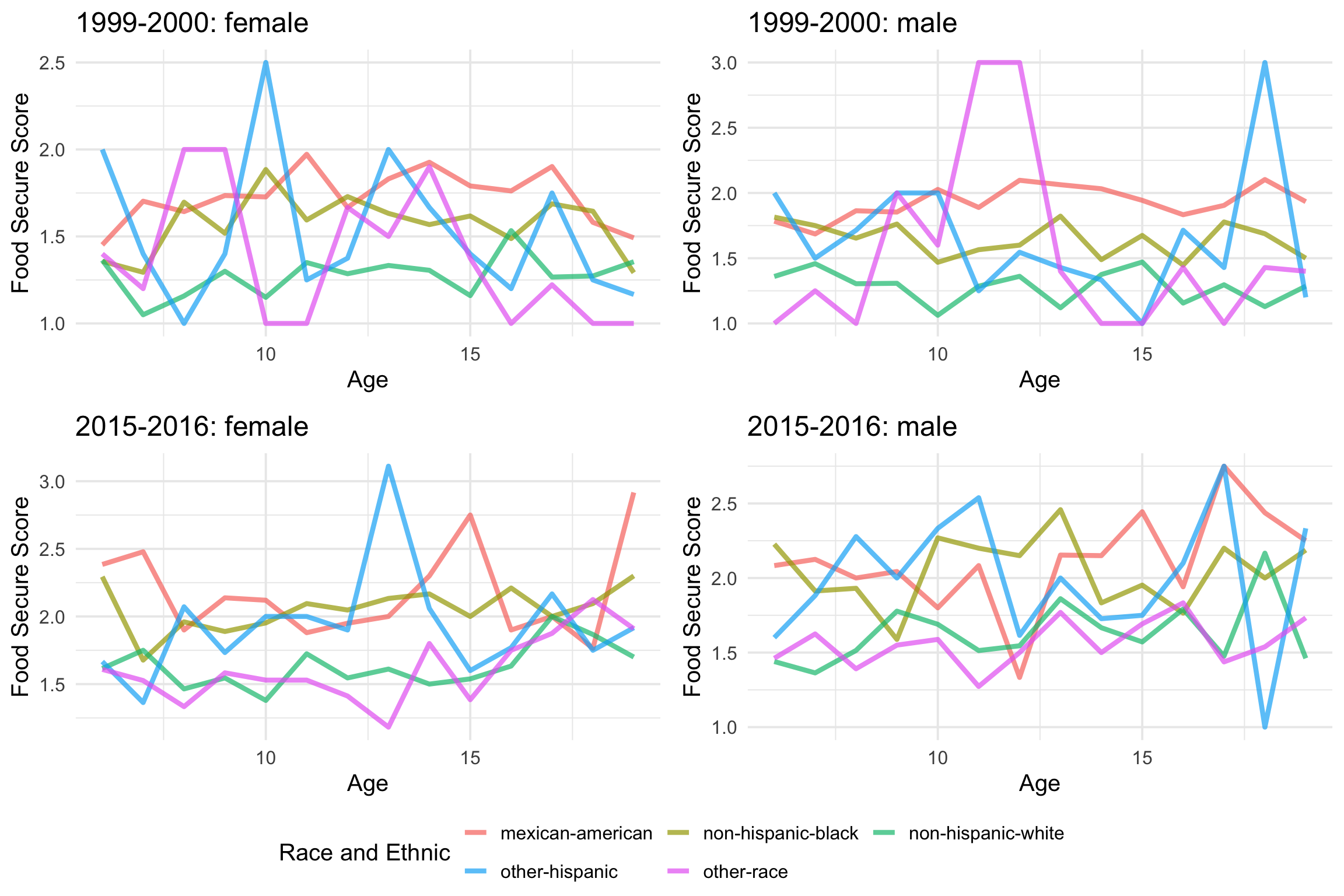
pmap_*
With pmap_*, we can easily use the above code to produce figures for each row. When using pmap_*, the first input is a list of column names that we need from the dataframe and the second input is the plotting function we used in the last part. The ..1, ..2, and ..3 are corresponding to data, gender, and year. Then, Voila, you have a figure for data from each row!
child_model_plot_df <- child_model_df %>%
  mutate(nest_plot = pmap(list(data, gender, year),
                          ~{plotting(..1, ..2, ..3)})
                          )

ggpubr::ggarrange(child_model_plot_df$nest_plot[[1]],
                  child_model_plot_df$nest_plot[[2]],
                  child_model_plot_df$nest_plot[[17]],
                  child_model_plot_df$nest_plot[[18]],
                  ncol = 2, nrow = 2,
                  common.legend = TRUE,
                  legend = 'bottom')
Another cool thing about nest, is that we can easily reverse this process with unnest after we finished our grouped analysis.
adult_df = model_df %>%
  filter(age_group == 'adult') %>%
  select(year, gender, age_group, data) %>% unnest(data)
head(adult_df)
# A tibble: 6 x 8
# Groups:   year, gender, age_group [1]
  year      gender age_group    id   age race_ethnic
  <chr>     <fct>  <fct>     <dbl> <dbl> <fct>
1 1999-2000 male   adult         2    77 non-hispanic-white
2 1999-2000 male   adult         5    49 non-hispanic-white
3 1999-2000 male   adult        12    37 non-hispanic-white
4 1999-2000 male   adult        13    70 mexican-american
5 1999-2000 male   adult        14    81 non-hispanic-white
6 1999-2000 male   adult        29    62 non-hispanic-white
# … with 2 more variables: hh_food_secure <dbl>, educ <dbl>
map2_*
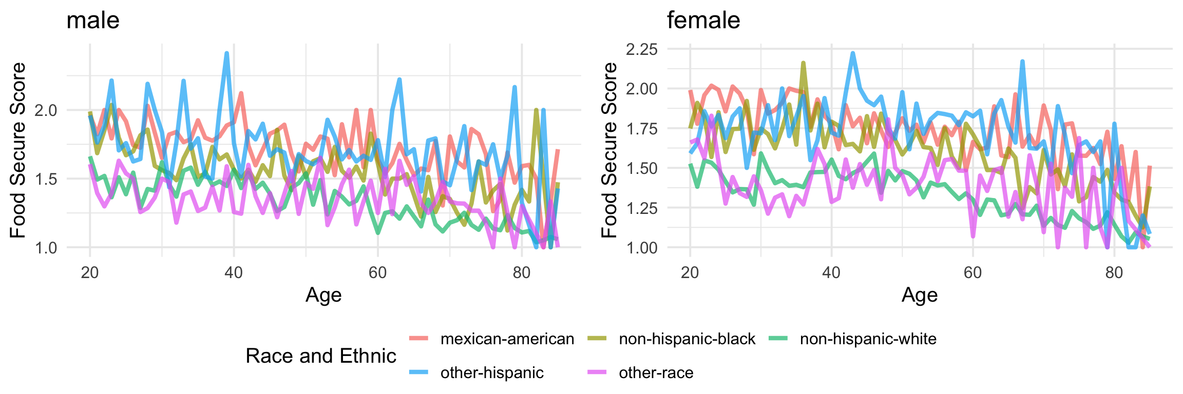
Lastly, once we learned about pmap_*, map2_* is very similar. Instead of being able to use as many variables you need with pmap, map2 is specialized for only 2 inputs. Let’s see an example below. Since we have found that the relationship between age and food security are pretty consistent over the years, let’s make a plot that ignore the age factor with map2.
adult_plot_df = adult_df %>%
  group_by(gender) %>%
  nest() %>%
  mutate(nest_plot = map2(data, gender,
                          ~plotting(.x, .y)))

ggpubr::ggarrange(adult_plot_df$nest_plot[[1]],
                  adult_plot_df$nest_plot[[2]],
                  ncol = 2,
                  common.legend = TRUE,
                  legend = 'bottom')